Energy-based Models for Grasp Planning

Abstract: State of the art grasp planning techniques use a two-stage approach in which scene information is fed to a grasp generator network and the sampled grasp is fed to an evaluator network to both estimate the probability of grasp success and refine the grasp. The key issue with these techniques is that the two stages are disjointed and act independently because no back propagation of gradients takes place between the two networks. This work is motivated by bridging the gap between grasp sampling, evaluation, and refinement with energy-based models. Given a scene, a grasp can be generated, evaluated, and refined in one shot by descending down the energy manifold. Using a contrastive approach, the energy-based model was trained on ~200,000 examples with a noise contrastive estimation loss function. Results suggest the energy-based model is able to generalize to new scenes, differentiate good from bad grasps, and generate viable grasps.

Introduction

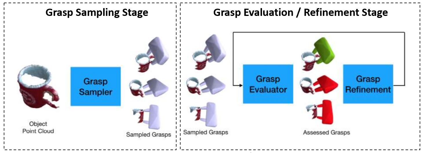
Grasping has been a long-standing challenge in robotics with a wide range of real-world application in manufacturing, logistics, and healthcare. Although much progress has been made toward improving generalizability of grasp planning techniques to novel objects over the past few years, the performance of such techniques is not yet at the level required for deployment in industry. State of the art grasp planning techniques [1]-[3] use a two-stage approach, as depicted in Figure 1, in which scene information is fed to a grasp generator network and the sampled grasp is fed to an evaluator network to both estimate the probability of grasp success and refine the grasp. The key issue with these techniques is that the two stages are disjointed and act independently because no back propagation of gradients takes place between the two networks. This work is motivated by bridging the gap between grasp sampling, evaluation, and refinement with energy-based models.

two-stage-approach — Figure 1: Two-stage approach for current state of the art grasp planning techniques (image obtained from Mousavian et al. [2])

Method

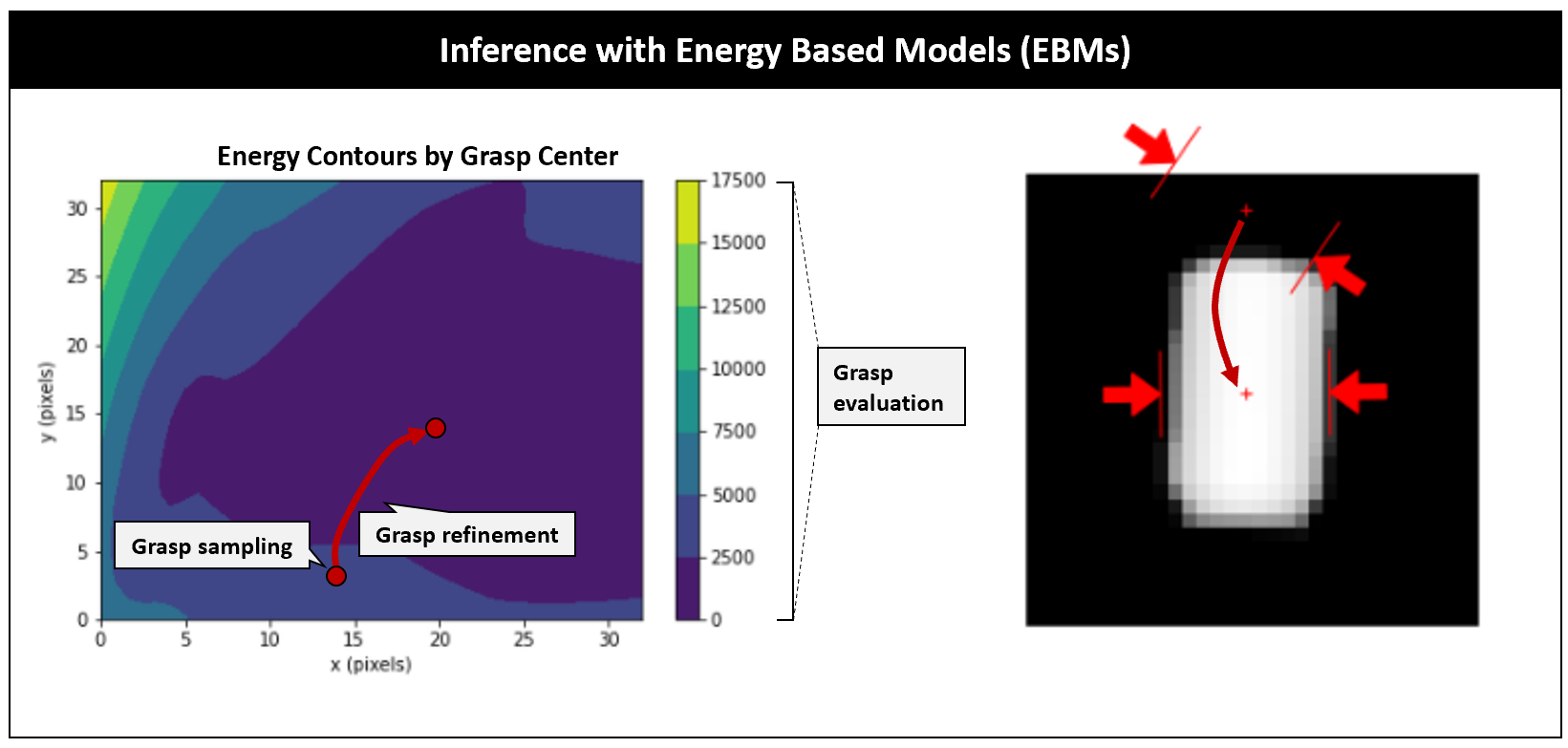
Energy-based models comprise of a surface manifold which associates high energy to negative samples and low energy to positive samples. In this work, a positive and negative sample is given by a grasp with a high and low probability of success respectively. Upon inference, a grasp can be sampled at random as shown in Figure 2. The energy of the sampled grasp is given by the energy manifold and is associated with the quality of the grasp. The sampled grasp can be refined by descending down the energy manifold towards regions of higher quality grasps. Grasps with relatively high probability of success are found at the local minima of the energy manifold. Note that the energy can be transformed into a probability of grasp success by the Gibbs-Boltzmann distribution but calculating the normalizing partition function may be intractable [4]. The energy formulation therefore allows for representation of complex distribution that may be difficult to represent with probabilistic methods.

ebm-inference — Figure 2: Inference with energy-based models for grasp planning such that grasps are sampled at random, evaluated by the energy value, and refined by descending down the energy manifold toward regions of higher quality grasps

Using a contrastive approach, the energy-based model can be trained by pushing up on energies of negative samples and pushing down on energies of positive samples. A wide variety of loss functions can be used for such a contrastive approach. In this work, the noise contrastive estimation loss function [5]-[7] given by

\[L = \frac{1}{n^+} \sum_{i=1}^{n^+} \ell_i\] \[\ell_i = \frac{E_w(x_i, y_i)}{\tau} + \log \left[\exp\left(\frac{-E_w(x_i, y_i)}{\tau}\right) + \sum_{j=1}^{n^-} \exp\left(\frac{-E_w(x_j, \hat{y}_j)}{\tau}\right)\right]\]

was used where \( L\) is the loss, \( \ell_i \) is the loss per positive sample, \( n^+\) is the number of positive samples, \( E_w(x_i, y_i) \) is the energy parameterized by \( w\) given a depth image \( x_i \) and a high-quality grasp \( y_i \), \( E_w(x_i, \hat{y_i}) \) is the energy given a depth image \( x_i \) and a low-quality grasp \( \hat{y_i}\), \( \tau \) is the temperature hyperparameter, and \( n^- \) is the number of negative samples in a given batch.

Experiment Setup

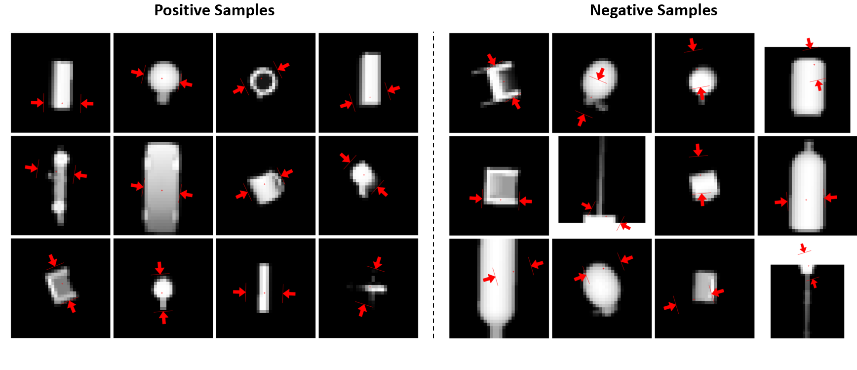
A subset of 220,000 examples from the Dexnet 2.0 dataset [1] was used for this work with a 90%/10% split for the training and validation set respectively. The Dexnet 2.0 dataset comprises of a synthetic dataset of 6.7 million depth images and grasps generated from 1,500 unique 3D object models. Figure 3 depicts a sample of the dataset for one object. Note that each depth image is 32 by 32 pixels with one channel while each grasp consists of a 4-dimensional grasp vector given by grasp center row, grasp center column, grasp depth, and grasp quality where grasp quality is a binary representation of grasp success, 1 for a positive sample with high probability of success and 0 for a negative sample low probability of success.

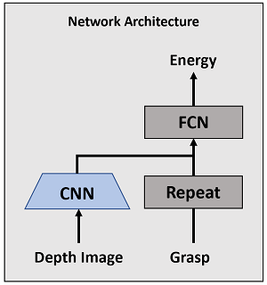
A relatively simple network architecture was used for the energy-based model as shown in Figure 4. The depth image is fed into a convolutional feature extractor comprising of four convolutional layers, each made up of a 2D convolution followed by a relu non-linearity and batch-normalization. The output channels for each layer are 16, 32, 64, and 64 channels respectively. The kernel size of all convolutions is 3 by 3 except for the first layer which has a size of 5 by 5. Similarly, the stride of all convolutions is 2 except for the first layer which has a stride of 1. All features outputted by the feature extractor are flattened into a 1028-dimensional vector. The grasp input is fed to a repeat module which simply expands the 4-dimensional input vector into 1028 dimensions by repeating the grasp vector 256 times. The resulting repeated vector is concatenated with the flattened feature extractor output before being fed into a four layer fully connected network with 2048, 512, 128, and 1 output activations respectively. Each layer of the fully connected network consists of a linear layer followed by a relu activation function and a dropout module. The final output of the network is the energy.

Several transformations were applied to the data before being fed into the network. During training, the grasp angle was first randomly rotated by 180 degrees with a probability of 0.5. This was done such that the resulting energy surface is symmetric across the grasp angle axis. Both the grasp and depth image were then normalized by subtracting from the mean and dividing by the standard deviation. During validation, only data normalization was applied.

In order to evaluate network performance throughout training, an alignment metric was monitored and defined as the percentage of positive samples with energy lower than any negative sample in a given batch. Note that throughout all experiments, a relatively large batch size of 512 samples was used to reduce loss and alignment variance. In addition, a learning rate of 1e-4 was used for all experiments.

Results

Figure 5 shows the resulting training curves after 500 epochs of training for 5 different experiments. Experiments only differ by the temperature hyperparameter chosen to study the impact of temperature on training and the resulting energy manifold.

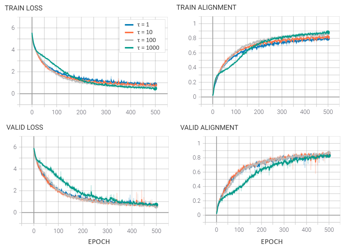
Table 1: Final model performance where τ is the temperature term in the noise contrastive estimation loss function
τ	Contrastive Loss	Alignment (%)
1	0.73	83.8
10	0.55	86.2
100	0.58	86.8
1000	0.69	82.8

Higher temperatures rescale the energy such that a larger number of negative samples contribute to the denominator of the loss function. In doing so, the system pushes up on multiple negative samples throughout each training iteration. The zero temperatures limit effectively yield a system that only pushes up on the most of offending negative sample with the lowest energy. Results suggest that \( \tau = 100 \) yields the best performance as highlighted in Table 1.

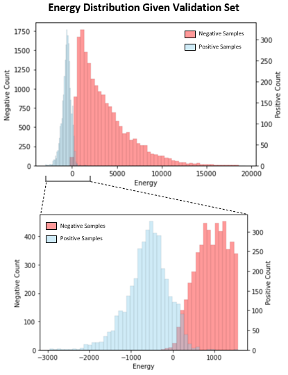
Figure 6 shows the outputted energy distribution for the validation set associated with the model trained with temperature equal to 100. Note that the two distributions started out similar but throughout training, the system was able to separate the two distributions by pushing up on energies of negative samples and pushing down on energies of positive samples through minimization of the contrastive loss.

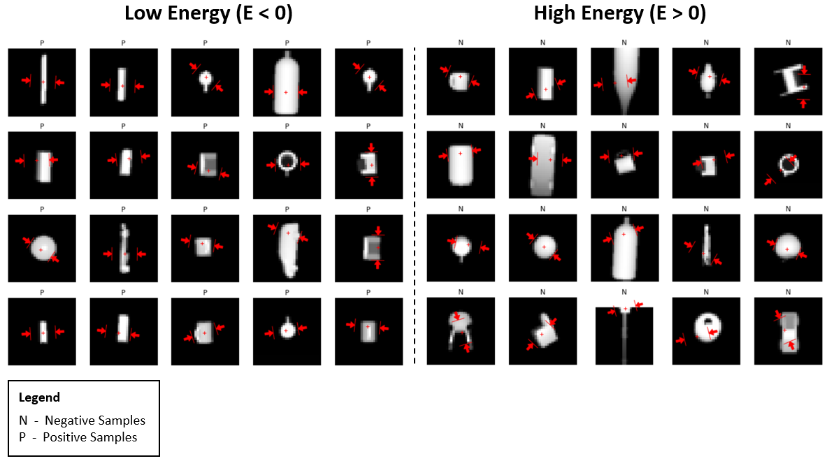
high-vs-low-energy — Figure 7: Sample set of depth image and grasp pairs associated with low energy (energy < 0) and high energy (energy > 0)

The left side of Figure 7 shows pairs of grasp and depth image associated with low energy while right side shows pairs associated with high energy. Note that high energies correspond to negative samples while low energies correspond to positive samples.

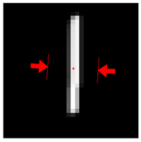
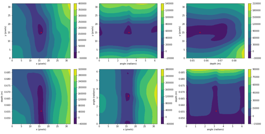
Now that we have a trained energy-based model, we can perform inference by sampling a grasp at random and descending down the energy manifold to a grasp with a high probability of success. Figure 9 shows contours of the energy manifold across different grasp dimensions centered on a valid or high-quality grasp marked as a red dot. The associated depth image and valid grasp is depicted in Figure 8. Note that the energy forms a local minimum near the region of the high-quality grasps. Also note that local minimum regions of the energy manifold are invariant to 180-degree rotations about the grasp axis as expected.

inference-example — Figure 8: Depth image and grasp pair associated with energy manifold contour shown in Figure 9

energy-contours — Figure 9: Energy manifold contours along various grasp axis associated with the depth image and grasp pair shown in Figure 8

The video below shows examples of grasp generation by gradient decent on the energy manifold. Note that the resulting grasps appear to be valid grasps.

Conclusion

We have shown that with energy-based models grasps can be samples, evaluated, and refined in one shot. By doing so, we have been able to bridge the gap between sampling, evaluation, and refinement stage that exists in current state of the art grasp planning techniques and yielded an integrated system. Results suggest the energy-based model is able to generalize to new scenes, differentiate good from bad grasps, and generate grasps that appear viable. The next step is to deploy the model in simulation to properly evaluate the probability of success of the generated grasps.

References

Jeffrey Mahler, Jacky Liang, Sherdil Niyaz, Michael Laskey, Richard Doan, Xinyu Liu, Juan Aparicio Ojea, and Ken Goldberg. “Dex-Net 2.0: Deep Learning to Plan Robust Grasps with Synthetic Point Clouds and Analytic Grasp Metrics.” Robotics, Science, and Systems, 2017. Cambridge, MA.
Arsalan Mousavian, Clemens Eppner, Dieter Fox. ”6-DOF GraspNet: Variational Grasp Generation for Object Manipulation.” International Conference on Computer Vision, 2019.
Adithyavairavan Murali, Arsalan Mousavian, Clemens Eppner, Chris Paxton, Dieter Fox. “6-DOF Grasping for Target-driven Object Manipulation in Clutter.” International Conference on Robotics and Automation, 2020.
Yann LeCun, Sumit Chopra, Raia Hadsell, Marc’Aurelio Ranzato, and Fu-Jie Huang. “A Tutorial on Energy-based Learning.” In G. Bakir, T. Hofman, B. Schölkopf, A. Smola, and B. Taskar, editors, Predicting Structured Data. MIT Press, 2007.
Michael Gutmann and Aapo Hyvӓrinen. Noise-contrastive estimation: A new estimation principle for unnormalized statistical models. In Proceedings of the Thirteenth International Conference on Artificial Intelligence and Statistics, pages 297–304, 2010.
Misra, I. and van der Maaten, L. Self-supervised learning of pretext-invariant representations. arXiv preprint arXiv:1912.01991, 2019.
Ting Chen, Simon Kornblith, Mohammad Norouzi, Geoffrey Hinton. “A Simple Framework for Contrastive Learning of Visual Representation.” International Conference on Machine Learning, 2020.